I recently read a fun paper Reed Solomon Codes over the Circle Group
that uses circle groups to perform an important kind of error correcting code in
finite fields where it’s otherwise difficult. If that sounds like gibberish to
you, be not afeard! That’s not really what I’m here to talk about! While quite
tangential to the contents of the paper, I was intrigued by the idea of
translating circle groups into the context of finite fields, and wondered if
there was a good way to understand these groups spatially, given how weird
finite fields tend to be. Hence the title of the blog post!
The Unit Circle
I started programming back in high school, around the same time I was learning
trigonometry. I really enjoyed making simple games and physics simulations, and
for one project I wanted to have a ball bouncing around the screen, starting in
a uniformly random direction. This led me to ask myself, “what should the velocity
of the ball be, given the angle I want it to go in?” I drew a right triangle,
chanted SOH-CAH-TOA, and landed on a solution that looked something like this:

The next week in math class, the teacher drew the same picture up on the board,
set \(v = 1\), and introduced something that blew my mind with how nicely it
tied together so many ideas: the unit circle. Fast-forward a bit further, and
we’re introduced to the complex plane, where the connections go even further:
our vector with an angle \((v\mathrm{cos}\theta, v\mathrm{sin}\theta)\) now
becomes a single complex number \(v\mathrm{cos}\theta + i v\mathrm{sin}\theta\).
This also lends a nice spatial understanding of complex multiplication: the
magnitudes (i.e. \(v\)) multiply, and the arguments (i.e. \(\theta\)) add,
which we can prove algebraically with a bit of trigonometry:
\[(v_1\mathrm{cos}\theta_1 + i v_1\mathrm{sin}\theta_1)(v_2\mathrm{cos}\theta_2 + i v_2\mathrm{sin}\theta_2) \\
= v_1 v_2 \mathrm{cos}\theta_1 \mathrm{cos}\theta_2 + i v_1 v_2 \mathrm{sin}\theta_1 \mathrm{cos}\theta_2 +
i v_1 v_2 \mathrm{cos}\theta_1 \mathrm{sin}\theta_2 + i^2 v_1 v_2 \mathrm{sin}\theta_1 \mathrm{sin}\theta_2 \\
= v_1 v_2 (\mathrm{cos}\theta_1 \mathrm{cos}\theta_2 - \mathrm{sin}\theta_1 \mathrm{sin}\theta_2) + i v_1 v_2 (\mathrm{sin}\theta_1 \mathrm{cos}\theta_2 + \mathrm{cos}\theta_1 \mathrm{sin}\theta_2) \\
= v_1 v_2 \mathrm{cos}(\theta_1 + \theta_2) + i v_1 v_2 \mathrm{sin}(\theta_1 + \theta_2)\]
If we take two points on the unit circle, their magnitudes are both 1, so the
magnitude of their product is \(1 \cdot 1 = 1\). This means that if we limit
ourselves to points on the unit circle, multiplying them gives us another point
on the unit circle. This property is called closure (under multiplication).
The complex unit circle has a couple of other properties that make it
interesting: multiplication by 1 leaves a point unchanged, and 1 is a point on
the unit circle. We call this point the multiplicative identity. Also, for
every point on the unit circle \(z\) there is another point \(z^{-1}\),
also on the unit circle, which we call the multiplicative inverse of \(z\),
such that \(z \cdot z^{-1} = 1\). In particular, if
\(z = \mathrm{cos}\theta + i \mathrm{sin}\theta\) then
\(z^{-1} = \mathrm{cos}\theta - i \mathrm{sin}\theta\), which also happens to
be the complex conjugate typically denoted \(\overline{z}\).
\[z \cdot z^{-1} = (\mathrm{cos}\theta + i \mathrm{sin}\theta)(\mathrm{cos}\theta - i \mathrm{sin}\theta) \\
= \mathrm{cos}^2\theta + i \mathrm{sin}\theta \mathrm{cos}\theta - i \mathrm{sin}\theta \mathrm{cos}\theta - i^2 \mathrm{sin}^2\theta \\
= \mathrm{cos}^2\theta + \mathrm{sin}^2\theta \\
= 1\]

So to summarize, the complex unit circle has the following interesting
properties: it is closed under multiplication, it contains a multiplicative
identity, and every point has a multiplicative inverse. Also, multiplication of
points on the unit circle is associative, because complex multiplication is
always associative. Structures with these properties are called groups, and
they show up all over the place in mathematics. Thus, the complex unit circle
under multiplication is a group.
It’s interesting to me that the unit circle is its own little closed “universe”
within the complex plane — much like the real numbers! This group is actually so
important that it’s usually just called the circle group. It turns out, we can
take it a lot further and find even smaller groups within the circle group. A
“group within a group” is called a subgroup, and we can find a lot of them —
intuitively, since multiplying complex numbers on the unit circle rotates us
around the circle, we can pick the number of points we want in our subgroup
(\(\ge 1\)), and place them evenly around the circle starting from 1. For
example, the subgroup of order 7 looks like this; notice how the points in the
subgroup are all \(\frac{360\degree}{7}\) apart on the circle.

What about finite fields?
Finite fields are near and dear to my heart. There are already tons of resources
about them just a Google search away, so I’ll keep the exposition brief.
Basically, the thing I found so cool about them was that all of arithmetic works
on these structures, despite having only finitely many elements. You can
sensibly add, subtract, multiply, and divide (except by zero), and things work
more or less how you would expect. They basically come in two flavors:
- Fields of prime order. That is, pick some prime number \(p\) — addition and
multiplication “wrap around” at \(p\). Subtraction and division are the
inverse operations. If we tried to use a non-prime value of \(p\), then
division breaks in the following way: suppose \(a\) and \(b\) are nonzero
factors of \(p\). Then \(a \cdot b = p = 0\), but dividing by \(a\)
implies \(a^{-1} \cdot a \cdot b = b = a^{-1} \cdot 0 = 0\) which is a
contradiction.
- Polynomials over fields of prime order. That is, pick some irreducible
polynomial with coefficients in the finite field — that means one that
doesn’t have any roots in the field. For example, over the field of order 5,
\(x^2 - 1 = (x + 4)(x + 1)\) is reducible because 1 and 4 are roots, whereas
\(x^2 + 1\) is irreducible. Addition and multiplication are modulo this
irreducible polynomial.
The complex numbers have a lot in common with this second flavor. When working
with the real numbers, some polynomials are factorable, like
\(x^2 - 1 = (x + 1)(x - 1)\) for example. Thus, \(x^2 - 1 = 0\) has the
solutions \(x = 1\) and \(x = -1\). Some polynomials are not factorable:
\(x^2 + 1 = 0\) has no real solutions, because \(x^2 + 1\) is always
positive; therefore, it is irreducible. In fact, if we relabel \(x\) as
\(i\), something interesting happens:
\[i^2 + 1 = 0 \\
i^2 = -1 \\
i = \sqrt{-1}\]
Although it’s a bit different from the way I learned it in my Algebra II class,
it’s equivalent to define the complex numbers as “univariate polynomials over
the real numbers modulo \(i^2 + 1\).” This also means that we can generalize
complex numbers to (most) finite fields by using the same irreducible polynomial,
and bring our definition of the unit circle along with us. Let’s define a
complex extension to be the field of univariate polynomials over a finite
field modulo \(i^2 + 1\). Also, if \(z = a + bi\) is an element of a complex
extension, then \(\overline{z} = a - bi\) is its complex conjugate. The
circle group of a finite field is the set of elements of its complex extension
satisfying \(z \cdot \overline{z} = 1\).
Okay, let’s draw some “circles”
There’s one last thing to attend to here, which is that finite fields are
discontinuous, by virtue of their finiteness. This means that if we plot two
points in our circle group, we can’t really draw a curve between them of points
that are also in our circle group. This makes it sort of tricky to think about
“going around” the circle like we can in the complex numbers. One natural remedy
to this would be to put the points in an order — but since the numbers wrap
around at the modulus, comparing our field elements like they’re integers means
inequalities don’t really work, and complex numbers aren’t even ordered either.
Luckily, there’s a useful tool from group theory that gives us a way to order
the elements of some finite groups like the circle group (the so-called cyclic
groups): generators. A generator is an element of the group whose powers
enumerate all the elements of the group. For our subgroup of order 7 in the
complex plane, we can write all the elements as powers of the element in the
first quadrant which I’ll call \(g\) for generator:

There’s another wrinkle here, in that there’s usually more than one generator,
which enumerate the points in different orders. For example, \(g^2\) is also
a generator, as we can see with a bit of arithmetic mod 7. This generator
“skips around” the circle by regular intervals, and traces out a star shape.
\[(g^2)^0 = g^0 \\
(g^2)^1 = g^2 \\
(g^2)^2 = g^4 \\
(g^2)^3 = g^6 \\
(g^2)^4 = g^8 = g^1 \\
(g^2)^5 = g^{10} = g^3 \\
(g^2)^6 = g^{12} = g^5\]
Clearly we need some way to pick a generator that enumerates the points in the
most “circle-like” way. Intuitively, this is \(g\): in the complex numbers
over the reals, it visits the points in counterclockwise order. \(g^2\), on
the other hand, “cuts across” the circle to make a more complicated shape. Thus,
I propose the heuristic of taking the generator that produces the circle with
the smallest perimeter to be the one we want. There are some major problems with
this, but this is no journal article and we’re here for some cool pictures, darn
it! The first issue is that neither finite fields nor their complex extensions
are metric spaces, and so there aren’t really coherent notions of length to lean
on; instead, we just blindly use Euclidean distance on the plots. The second
issue is that the way we choose to present the circles affect these distances.
I decided to make these plots with axes ranging from \(-\frac{p}{2}\) to
\(\frac{p}{2}\), but I could equally well have made them range from 0 to
\(p\). I made this choice so that the plots are centered on 0 like in the
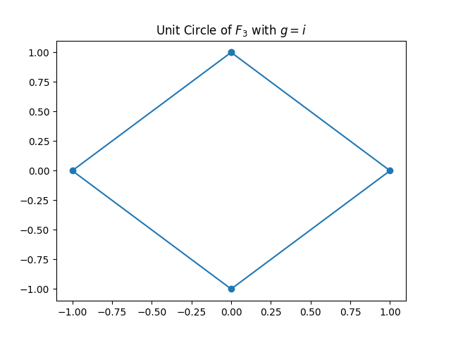
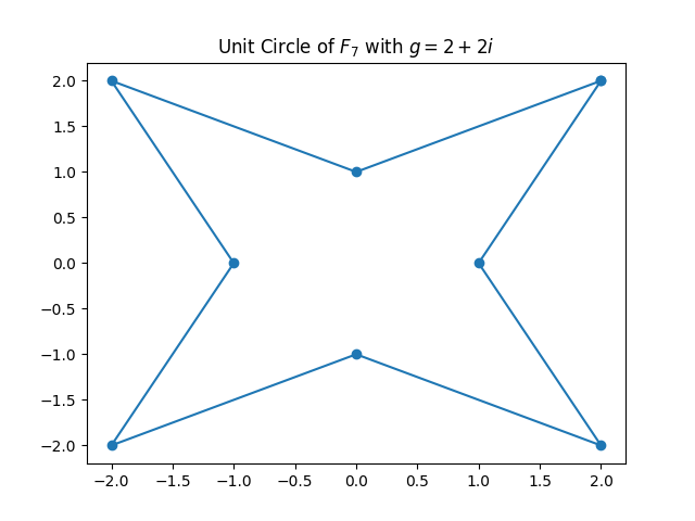
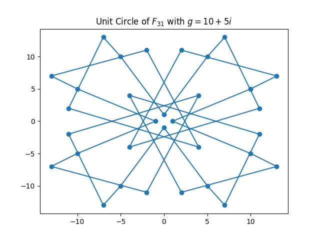
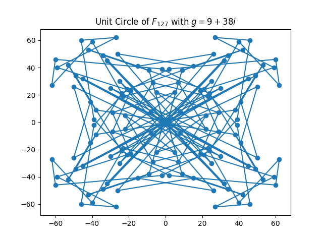
traditional complex unit circle. Without further ado, here are the unit circles
for the first few Mersenne primes, as considered in the paper by Haböck et al.