Maybe you’ve seen cool engineering graphics like this one before. This is a
model of heat computed over a 3D model of a mechanical part. I wanted to
understand how to make these kinds of simulations myself, and seeing as most of
the actual theory was hidden away in textbooks and lecture notes, I thought I’d
try to create the kind of resource I wish I’d found while trying to learn this
stuff. While I have also explored the 2D and 3D flavors of this technique which
I may write up in the future, we’ll stick to 1D for the remainder of this post
to keep things simple.
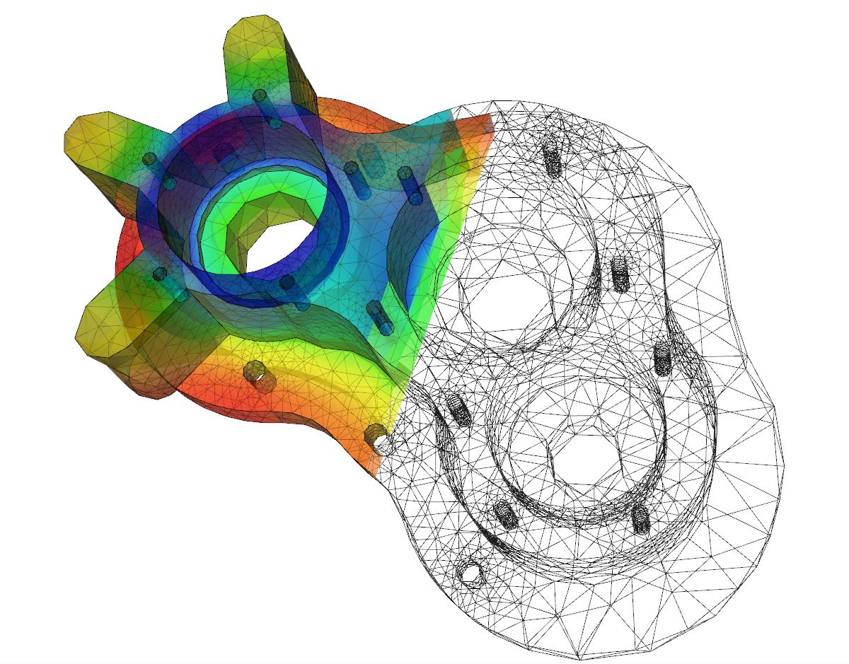 "Visualisation of heat transfer in a pump casing" by User A1 at Wikimedia Commons, licensed under
CC BY-SA 3.0
"Visualisation of heat transfer in a pump casing" by User A1 at Wikimedia Commons, licensed under
CC BY-SA 3.0
The Problem
The finite element method (FEM) is fundamentally a computational method for
finding approximate solutions to differential equations. Differential equations
pop up all over the place in the physical sciences — in physics, Newton’s second
law, Maxwell’s equations, and the Schrödinger equation sit at the core of
classical mechanics, electromagnetism, and quantum mechanics, respectively. In
chemistry, they appear in models of kinetics and diffusion, and in engineering
they model heat, fluids, and the deformation of solids. All of these offer
potential applications of FEM, but it’s this last one — deformation of solids —
that we’ll be focusing on here.
Differential equations are equations that describe the relationship between a
function and its derivatives. With “regular” equations, you “solve for \(x\)”
to find the previously unknown number, whereas with differential equations you
“solve for \(f\)” to find the previously unknown function. Typically, there are
a lot of different functions that satisfy a particular differential equation,
and so typically we will want to also satisfy some boundary conditions: extra
properties that narrow down the result to the particular one that we want, such
as passing through a particular point or having a particular slope somewhere.
Depending on the boundary conditions, differential equation problems generally
fall into one of two categories. The first, and I think easier to understand, is
called an initial value problem (IVP). For example, in Newtonian mechanics
you’re typically given the complete state of the system at some point in time —
for one particle, an instantaneous position and velocity suffices. Then Newton’s
second law (the differential equation) allows you to compute the acceleration
from the position and velocity. Since velocity is the derivative of position and
acceleration is the derivative of velocity, one can approximate the state of the
system a short amount of time \(\Delta t\) later as \(\vec{v} = \vec{a} \Delta t\)
and \(\vec{r} = \vec{v} \Delta t\), and repeating this to reach an approximate
state at any future time. It’s a basic result of calculus that choosing \(\Delta t\)
to be small enough, it’s possible to get arbitrarily close to the exact state.
This procedure, called the “forward Euler method,” works for any IVP, since a
complete description at one point in the domain tells you about the behavior at
nearby points. There are, of course, more accurate methods for approximating
solutions, but hopefully the forward Euler method gives some good intuition for
why this case is “special.”
The other class of differential equation problems are called boundary value
problems (BVPs). Here, the boundary conditions are spread out over two or more
points in the domain, but with an incomplete description at any particular one
of them. Using Newtonian mechanics for an example again, we might know the
position of the particle at the beginning of some time interval and its velocity
at the end, or vice versa. The important thing to note here is that the forward
Euler method fundamentally doesn’t work here, at least not like it did before.
If we know the initial position but not velocity, we can’t reliably estimate its
position after \(\Delta t\). At best, we can guess the initial velocity,
integrate, and see if the result lines up with the other boundary condition at
the end, and iterate until we find an acceptably close solution — this approach
is called “the shooting method,” which I take as an analogy for aiming a cannon
by firing blind, looking where the cannonball landed, and adjusting until you
hit the target. FEM is a more refined approach to this problem.
The Theory
The finite element method approaches BVPs by turning them into linear algebra
problems. Unfortunately, the solutions to differential equations can generally
be any sufficiently smooth real-valued function over the appropriate interval,
which forms an infinite dimensional vector space (consider as a basis the set of
monomials \(f_i(x) = x^i\), all of which are smooth functions). Working with
infinitely long vectors is not feasible, so instead we’ll need a finite
dimensional approximation. To this end, let \(\Omega\) be the closed interval
\([a, b]\) we’re solving over, and let \(M \subseteq \Omega\) be a finite subset
that contains the endpoints, which we call the mesh. For notational
convenience, we index the elements of \(M\) in order, so that
\(x_0 < x_1 < \ldots < x_{|M|-1}\).
Since I’m primarily interested in second order differential equations, i.e.
those involving up to second derivatives of the unknown function, and because
of an “order reduction trick” we’ll see in a minute, it’s practical to work with
continuous piecewise linear functions. We can pick our basis to be the tent
functions over \(M\), which will turn out to be a very convenient choice:
\[\begin{align*}
T_{x_i}(x) &\coloneqq \begin{cases}
\frac{x - x_{i-1}}{x_i - x_{i-1}} & \mathrm{if} & x_{i-1} < x < x_i \\
\frac{x_{i+1} - x}{x_{i+1} - x_i} & \mathrm{if} & x_i \le x < x_{i+1} \\
0 & \mathrm{otherwise} \\
\end{cases} \\
T_{x_i}'(x) &= \begin{cases}
\frac{1}{x_i - x_{i-1}} & \mathrm{if} & x_{i-1} < x < x_i \\
\frac{-1}{x_{i+1} - x_i} & \mathrm{if} & x_i < x < x_{i+1} \\
0 & \mathrm{if} & x < x_{i-1} \vee x_{i+1} < x \\
\end{cases} \\
\end{align*}\]
Note that the ends of our interval \(x_0 = a\) and \(x_{|M|-1} = b\) have no
left or right neighbor, respectively, but these would only be necessary to
define these functions outside their domain, so we take them to be “cut off” —
so-called half tent functions. The tent functions generally look like this,
ramping up and down linearly from 0 to 1 back to 0. Notably, each of these
functions is 1 at a unique mesh point and 0 at all others.
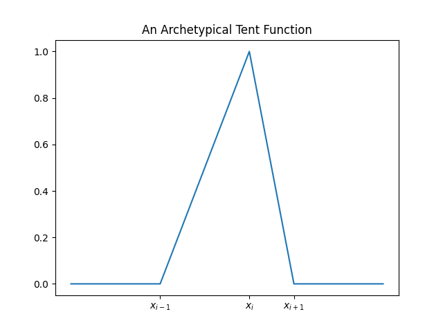
This gives us an \(|M|\)-dimensional vector space of continuous, piecewise linear
functions, which can approximate functions reasonably well with a careful choice
of the mesh \(M\) — this will be one of the tunable parameters when using FEM in
practice. We call this vector space \(P_1(M)\). Given a function
\(f : \mathbb{R} \rightarrow \mathbb{R}\), it’s easy to find a projection
\(\pi : (\mathbb{R} \rightarrow \mathbb{R}) \rightarrow P_1(M)\) that gives a
function in our new space that agrees at every point in \(M\):
\[\pi f(x) = \sum_{x_i \in M} f(x_i) \cdot T_{x_i}(x)\]
Now solving the BVP basically amounts to finding a good approximation of the
“true” solution in this finite dimensional vector space. One big problem though
is that these piecewise linear functions aren’t differentiable at points in
\(M\), and at any other point their second derivatives are always zero! Like I
said, we need a “degree reduction trick” to get around this, which is to switch
to a weak formulation of the differential equation. The particulars of this
vary a bit depending on the exact structure of the equation to be solved, but
the core idea is that if we have a general second order differential equation
for an unknown function \(u(x)\) of the form
\[\mathcal{F}(x, u, u', u'') = f(x)\]
we can introduce a test function \(v(x)\), and for any \(u\) that satisfies
the differential equation it must also be the case that
\[\int_\Omega \mathcal{F}(x, u, u', u'') v(x) \mathrm{d}x = \int_\Omega f(x) v(x) \mathrm{d}x\]
Note that \(u\) satisfying the first equation means that it necessarily
satisfies the second equation, but not necessarily the other way around. That’s
why we call the second equation a “weak formulation.” This is also sort of the
point: piecewise linear functions aren’t usually solutions to “interesting”
second order differential equations, which is precisely why we switched to the
weak formulation in the first place. It turns out, though, that piecewise linear
weak solutions are the best possible approximations in \(P_1(M)\) of the “true”
strong solution, at least in some sense. I’ll say more about this later, but
first let’s discuss the mechanics of the method.
The next step is to eliminate \(u''\) from the left side of the equation using
integration by parts. If \(F(x, u, u', u'')\) is nonlinear in a way that makes
this impossible, then we would need to employ more sophisticated strategies like
using piecewise quadratic basis functions or linearization. If integration by
parts works, though, we end up with a lower order functional \(\mathcal{A}\) and
a boundary term \(r(x, u, u')|_{\partial\Omega}\), which gives something of the
form
\[\int_\Omega \mathcal{A}(x, u, u') v'(x) \mathrm{d}x = \int_\Omega f(x) v(x) \mathrm{d}x + r(x, u, u')|_{\partial\Omega}\]
The general procedure from here is to choose \(v\) to be a basis function, and
express \(u\) in terms of a linear combination of basis functions. This turns
the left side of our weak formulation equation into an integral of sums, which
can be interchanged into sums of integrals of our basis functions. These
integrals give rise to the stiffness matrix \(A\) of the system, where the
form of the stiffness matrix depends on the particular form of the functional
\(\mathcal{A}\). On the other side of the equation, we have the integral that
gives rise to the load vector:
\[b_i = \int_\Omega f(x) T_{x_i}(x) \mathrm{d}x\]
In deriving the stiffness matrix, we take \(u(x) \in P_1(M)\), and therefore a
linear combination of basis functions
\[u(x) = \sum_{x_i \in M} \xi_i T_{x_i}(x)\]
Which gives the linear system
\[A \vec{\xi} = \vec{b} + \vec{r}\]
We have obviously glossed over a lot of gaps here that will need to be filled in
with more specific details for the particular problems we want to solve, so in
the next section we’ll work an example.
A 1D Linear Rod
Like I said before, my original motivation for learning FEM was to study the
deformation of solids, so all of the examples will follow in that vein. The
first system is really simple: consider a one meter long bar. Fix the left end
at the origin, and point the bar along the \(+x\) axis. Apply a force \(F\) at
the right end, which will stretch or compress the bar so that the right end is
no longer quite at the one meter mark.
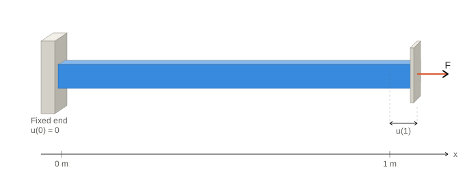
To model this system, we’ll need to introduce material coordinates: let this
coordinate \(X\) range from 0 to 1 meter, and correspond to the part of the bar
that “started out” at that position before the force was applied. For example,
\(X=0\) is the left end of the bar, \(X=1\) is the right end of the bar, and in
general there’s some displacement \(u(X)\) that tells us how far the piece of
the bar at \(X\) is from where it started. This means that \(x = X + u(X)\).
We’ll consider the bar to be a linearly elastic material — any material can be
approximated this way for sufficiently small deformations, but this assumption
breaks down for large deformations. The stiffness depends on the material, which
amounts to a material property called the Young’s Modulus \(E\), and the
cross-sectional area of the bar. The stiffness of the bar grows linearly with
both, so we’ll reduce them to a single quantity that may vary over the length of
the bar \(\mathrm{EA}(X)\). You could imagine this quantity varying because the
bar is thicker in some places than others, or because the material itself is
different in different parts of it.
If the internal load on the bar, which might include the weight of the bar
itself, is given by \(f(X)\), then we have this equation for the balance of
forces:
\[\frac{\mathrm{d}}{\mathrm{d}X} \left[ \mathrm{EA}(X) \frac{\mathrm{d}u}{\mathrm{d}X} \right] = -f(X)\]
Together with the boundary conditions that the left end of the bar is fixed at
the origin and the force at the right end is equal to \(F\).
\[\begin{align*}
u(0) &= 0 \\
u'(1) &= \frac{F}{\mathrm{EA}(1)} \\
\end{align*}\]
For any test function \(v(X)\), we have the weak formulation
\[\int_0^1 \frac{\mathrm{d}}{\mathrm{d}X} \left[ \mathrm{EA}(X) \frac{\mathrm{d}u}{\mathrm{d}X} \right] v(X) \mathrm{d}X
= -\int_0^1 f(X) v(X) \mathrm{d}X\]
The left side, notably, is amenable to integration by parts. Since we have the
essential boundary condition \(u(0) = 0\), we also take \(v(0) = 0\), and use
the other boundary condition to rewrite in terms of \(F\):
\[\begin{align*}
\int_0^1 \frac{\mathrm{d}}{\mathrm{d}X} &\left[ \mathrm{EA}(X) u'(X) \right] v(X) \mathrm{d}X \\
&= \left[ \mathrm{EA}(X) u'(X) v(X) \right]\big|_0^1 - \int_0^1 \mathrm{EA}(X) u'(X) v'(X) \mathrm{d}X \\
&= F v(1) - \int_0^1 \mathrm{EA}(X) u'(X) v'(X) \mathrm{d}X
\end{align*}\]
The term \(F v(1)\) is what ultimately enforces the second boundary condition,
and defines the \(\vec{r}\) vector in the vector equation we’re after so we’ll
move it over to the other side of the equation. We now have
\[\int_0^1 \mathrm{EA}(X) u'(X) v'(X) \mathrm{d}X = \int_0^1 f(X) v(X) \mathrm{d}X - F v(1)\]
Now taking \(v(X) = T_{x_i}(X)\) for any \(x_i \in M\) and
\(u(X) = \sum_{x_j \in M} \xi_j T_{x_j}(X)\), we have
\[\begin{align*}
&\int_0^1 \mathrm{EA}(X) \left[ \sum_{x_j \in M} \xi_j T_{x_j}'(X) \right] T_{x_i}'(X) \mathrm{d}X
= \int_0^1 f(X) T_{x_i}(X) \mathrm{d}X - F T_{x_i}(1) \\
\iff &\sum_{x_j \in M} \xi_j \left[ \int_0^1 \mathrm{EA}(X) T_{x_j}'(X) T_{x_i}'(X) \mathrm{d}X \right]
= \int_0^1 f(X) T_{x_i}(X) \mathrm{d}X - F T_{x_i}(1)
\end{align*}\]
And so if we set
\[\begin{align*}
A_{ij} &= \int_0^1 \mathrm{EA}(X) T_{x_j}'(X) T_{x_i}'(X) \mathrm{d}X \\
b_i &= \int_0^1 f(X) T_{x_i}(X) \mathrm{d}X - F T_{x_i}(1)
\end{align*}\]
we get the matrix equation we’re after:
\[A \vec{\xi} = \vec{b}\]
Another thing worth noting is that each of our tent functions is only nonzero
on a small part of the domain. In particular, the function \(T_{x_i}\) is only
nonzero between \(x_{i-1}\) and \(x_{i+1}\). Thus, \(T_{x_i}(X) T_{x_j}(X)\) is
nonzero only if \(x_i\) and \(x_j\) are identical or neighbors in \(M\), which
means \(A_{ij}\) is nonzero only on the diagonal and just above or below.
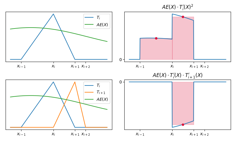
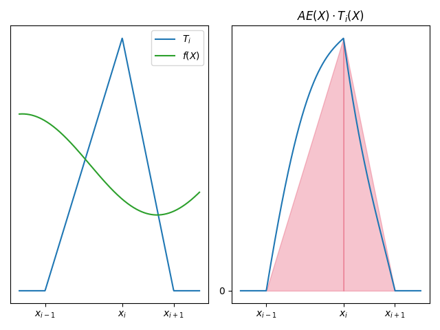
Depending on the particular functional form of \(EA(X)\), these integrals may be
difficult to evaluate. However, a reasonable closed-form approximation can be
obtained using a midpoint approximation. The figure below illustrates an example
function \(\mathrm{AE}(X)\) for “on-diagonal” and “off-diagonal” entries in the
stiffness matrix. The subplots on the left show the plot of \(\mathrm{AE}(X)\)
alongside the relevant basis functions, while the subplots on the right show the
integrand itself alongside the area computed by the approximation. Note that the
approximation is exact if \(\mathrm{AE}(X)\) is linear over the relevant
intervals, and the error vanishes as the relevant interval shrinks to zero.
Thus, by choosing \(M\) to have small intervals where the function has
larger second derivatives makes this approximation more accurate.
\[\begin{align*}
A_{ii} &\approx \frac{\mathrm{AE}\left(\frac{x_{i-1} + x_i}{2}\right)}{x_i - x_{i-1}}
+ \frac{\mathrm{AE}\left(\frac{x_{i} + x_{i+1}}{2}\right)}{x_{i+1} - x_{i}} \\
A_{i+1,i} = A_{i,i+1} &\approx -\frac{\mathrm{AE}\left(\frac{x_i + x_{i+1}}{2}\right)}{x_{i+1} - x_i}
\end{align*}\]
For the load vector, we have a different integral, and will instead use the
trapezoid approximation, despite its generally worse accuracy than the midpoint
approximation, because \(T_{x_i}(x_{i-1}) = T_{x_i}(x_{i+1}) = 0\), which means
we can get away with only evaluating \(f(X)\) at a single point per entry.
Unlike the midpoint approximation, this is only exact if \(f(X)\) is constant
over the relevant intervals, but the error still vanishes as the interval
shrinks. Thus, by choosing \(M\) to have small intervals where the function has
large first derivatives makes this approximation more accurate.
\[\begin{align*}
b_i &\approx \frac{1}{2} (0 + f(x_i))(x_i - x_{i-1}) + \frac{1}{2}(f(x_i) + 0)(x_{i+1} - x_i) + FT_{x_i}(1) \\
&= \frac{f(x_i)(x_{i+1} - x_{i-1})}{2} + FT_{x_i}(1)
\end{align*}\]
With that, we have everything we need to set up our FEM solver for our 1D linear
rod problem. Let’s pick a particular problem that’s interesting enough to
showcase the properties of the solver, but simple enough to still have an
analytic solution. I choose:
\[\begin{align*}
\mathrm{AE}(X) &\coloneqq \kappa (1 + X) \\
f(X) &\coloneqq 0
\end{align*}\]
Which happens to have the analytic solution
\(u(X) = \frac{F}{\kappa} \ln (1 + X)\)
The Numpy library makes it really easy to solve linear systems in Python, and
is reasonably well optimized behind the scenes so it makes a great foundation to
build on. Here’s the full script for the 1D solver.
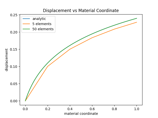
Here’s the resulting plot, showing the solver’s solution for 5 and 50 evenly
spaced segments. If you look closely, you can see the analytic solution is in
there too, hiding underneath the solution with 50 elements which is incredibly
accurate.
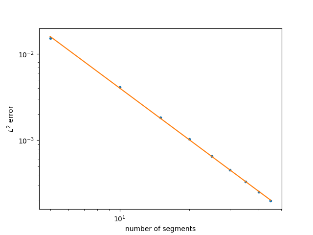
Because we have an analytic solution to compare against, we can plot a measure
of the absolute error (I went with the \(L^2\) norm, or root-mean-square error)
against the number of segments. Theoretically, the error should decrease
quadratically as the number of segments increases, and indeed we see a line with
approximately slope -2 in log-log space:
Why does this work?
In the last section, we set up a simulation of a 1D linear rod, and solved it
using the finite element method. For that particular example, which we were
able to compare against a known analytic solution, we were able to see that the
simulation produced very good approximations, and that the error vanished
quadratically with finer meshes. This is hopefully convincing evidence that the
method does work, but it’s definitely useful to understand why it works. After
all, I haven’t said anything so far that should convince you that weak solutions
should look anything like strong solutions.
Let \(u\) be a strong solution to the differential equation, and let \(u_{P_1}\)
be a weak solution. The weak solution satisfies this equation we got after
integrating by parts for any \(v \in P_1(M)\):
\[\int_0^1 \mathrm{EA}(X) u_{P_1}'(X) v'(X) \mathrm{d}X = \int_0^1 f(X) v(X) \mathrm{d}X - F v(1)\]
Meanwhile, the strong solution is also a weak solution, and therefore
\[\int_0^1 \mathrm{EA}(X) u'(X) v'(X) \mathrm{d}X = \int_0^1 f(X) v(X) \mathrm{d}X - F v(1)\]
The error of the weak solution is definitionally \(e(X) = u(X) - u_{P_1}(X)\),
and we can subtract the two equations above to obtain
\[\int_0^1 \mathrm{EA}(X) e'(X) v'(X) \mathrm{d}X = 0\]
The left side of this expression is a very convenient kind of thing called a
bilinear form. One of the nice properties of bilinear forms is that they induce
a notion of distance, or in the language of linear algebra a norm. This notion
of distance defines the sense in which the weak solution is “close” to the
strong solution, and in problems like this it usually corresponds to some notion
of energy. For our 1D linearly elastic rod in specific, this bilinear form is
\[a(f, g) \coloneqq \int_0^1 \mathrm{EA}(X) f'(X) g'(X) \mathrm{d}X\]
and the induced norm is
\[\|\cdot\|_a \coloneqq \sqrt{a(\cdot, \cdot)}\]
It’s worth taking a moment here to interpret this: \(\|u\|_a^2\) is the integral
of the rigidity of the rod multiplied by \(u'^2\) over the length of the rod.
This looks an awful lot like the equation for the potential energy of a spring,
\(\frac{1}{2}k(\Delta x)^2\), which is not a coincidence at all; this integral
is the strain energy of the deformed rod, up to a constant factor. Since a norm
is non-negative, a constant factor or squaring doesn’t affect the result of an
optimization problem. Thus, the function with the smallest value of
\(\|\cdot\|_a^2\) is the one that minimizes the overall strain energy of the rod
while still satisfying the boundary conditions.
Now let’s show that \(u_{P_1}\) is actually this function. Consider any other
function \(v_{P_1}(X) \in P_1(M)\), and let \(\delta = u_{P_1} - v_{P_1}\) which
is also in \(P_1(M)\). Observe that
\[u - v_{P_1} = u - u_{P_1} + u_{P_1} - v_{P_1} = e + \delta\]
Now consider the norm, and expand by linearity, noting that \(e\) is orthogonal
to \(\delta\) since it’s orthogonal to everything in \(P_1(M)\):
\[\begin{align*}
\|u - v_{P_1}\|_a^2
&= \|e + \delta\|_a^2 \\
&= a(e + \delta, e + \delta) \\
&= a(e, e + \delta) + a(\delta, e + \delta) \\
&= a(e, e) + \cancel{2a(e, \delta)} + a(\delta, \delta) \\
&= \|e\|_a^2 + \|\delta\|_a^2
\end{align*}\]
Finally, the punchline: convert this to an inequality, drop the \(\delta\) term,
and take the square root of both sides:
\[\|e\|_a = \|u - u_{P-1}\|_a \le \|u - v_{P_1}\|_a\]
Thus, the weak solution has the smallest error of any function in \(P_1(M)\), at
least as measured by this particular induced norm. In particular, the weak
solution has the lowest possible potential energy of any function in our finite
dimensional function space that satisfies the boundary conditions.
This tells us something else interesting: the function space \(P_1(M)\) is a
subspace of the full infinite dimensional space the strong solution lives in.
The strong solution has the smallest possible potential energy of any function
in that larger space, including our weak solution. Thus, weak solutions always
err on the side of having slightly higher potential energy, never lower, so the
finite element method always predicts structures to be slightly stiffer than
they really are.
Thanks for reading!